Adventures in Computing: Family Facial Recognition
One of the most common applications of machine learning is facial recognition. Plenty of examples of this exist, including Apple’s face unlock for iPhone, Windows Hello, and Google’s clustering of faces in the Google Photos app. I thought it would be fun to build something that could find my daughter’s face in family pictures, using just the data that I have. Incidentally, here is how much media I have with her in it:

Should be easy, right? Well, doing it well and understanding it took a week or two (mostly in the evenings after work and grading student’s homework for the class I teach).
Training Pipeline
The central idea is that I wanted to build an image processing pipeline. There are two parts to this: a training pipeline, and a classification pipeline.
Generating image chips
Step one is collecting data for training the classifiers. This was pretty easy, as I have years of family pictures on my hard drive:
chris@dijkstra [12:58:56 PM] [~]
-> % du -mach ~/Pictures/family --max-depth=1 | grep total
44G	total
chris@dijkstra [12:59:04 PM] [~]
-> %
Plenty of images there to train on. The first piece of code is an image chipper. Because the important part of an image is where the face is, we want to get labeled data where the faces are. This is done by chipping the image, extracting a subset of the image where interesting features are. For this I used scikit-learn’s Haar Cascade detector to find regions likely to contain a face. Cascade classifiers aren’t intuitively designed for facial recognition (you could use cascade classification to find cars, for example), so part of setting up the detector is choosing the configuration:
In [1]: import magic
   ...: import skimage.io as skio
   ...: from skimage import data
   ...: from skimage.color import gray2rgb, rgba2rgb
   ...: from skimage.feature import Cascade

In [2]: %pylab
Using matplotlib backend: Qt5Agg
Populating the interactive namespace from numpy and matplotlib

In [3]: detector = Cascade(data.lbp_frontal_face_cascade_filename())

In [4]: img = skio.imread("IMG_20200904_173228.jpg")

In [5]:
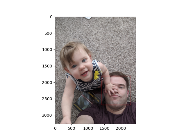
For demonstration purposes, we’ll use a picture of me and Evelyn, my daughter:
In [5]: plt.imshow(img)
Out[5]: <matplotlib.image.AxesImage at 0x7f1ca67ec4c0>

In [6]:
For the cascade detector, the user has to define the scale, step ratio, and min/max sizes. A variety of cameras and image resolutions are present in the dataset, so we’ll have a fairly large sweep range:
In [6]: detections = detector.detect_multi_scale(
   ...:     img,
   ...:     scale_factor=1.1,
   ...:     step_ratio=2.0,
   ...:     min_size=(100, 100),
   ...:     max_size=(2000, 2000),
   ...: )

In [7]: detections
Out[7]: [{'r': 1887, 'c': 1442, 'width': 854, 'height': 854}]

In [8]:
Detections are returned as the location of the upper left pixel (r
is a row, and c is a column), the width, and the height. Plotting
the single detection (later on we’ll discuss why it didn’t detect both
faces) shows that the detector found my face pretty well:
In [8]: detection = detections[0]

In [9]: x = detection["c"]
   ...: y = detection["r"]
   ...: height = detection["height"]
   ...: width = detection["width"]

In [10]: plt.gca().add_patch(
           patches.Rectangle((x, y), width, height, edgecolor="red", facecolor="none")
         )
Out[10]: <matplotlib.patches.Rectangle at 0x7ff544597d00>

In [11]:
This is enough to get us a good dataset. For this I wrote a program
called chipper.py, which recursively searches an image directory and
chips faces out of all of the images it finds. The main loop looks
like this:
for path in tqdm(image_paths):
	# We're skipping already chipped images
	if list(args.output_dir.glob(f"{path.name}.chip.*.png")):
		continue

	# If something goes wrong, just toss that image out and continue
	try:
		img = skio.imread(path)
	except SyntaxError:
		print(f"SyntaxError on {path}")
		continue
	except OSError:
		print(f"OSError on {path}")
		continue
	except ValueError:
		print(f"ValueError on {path}")
		continue

	# Use RGB images for the face detector
	if img.shape[-1] == 4:
		img = rgba2rgb(img)
	elif img.shape[-1] == 2:
		img = gray2rgb(img)

	detections = detector.detect_multi_scale(
		img,
		scale_factor=1.1,
		step_ratio=2.0,
		min_size=(100, 100),
		max_size=(2000, 2000),
	)
	for index, detection in enumerate(detections):
		x = detection["c"]
		y = detection["r"]
		height = detection["height"]
		width = detection["width"]
		with warnings.catch_warnings():
			warnings.filterwarnings("ignore", category=UserWarning)
			skio.imsave(
				args.output_dir / f"{path.name}.chip.{index}.png",
				img[y : y + height, x : x + width],
			)
Very simple, although searching through 40+ GB of images does take a little while.
Building a dataset
Once the images have all been chipped, I labeled them by placing them
into labeled folders corresponding to the person whose face was in the
chip. I also created a not_a_face label, to ensure there would be
non-face examples in the training set.
To combine images into a usable dataset, I decided to use HDF5 to create a portable dataset with lower memory requirements. An HDF5 file has random access to the on-disk data, so a pipeline that would otherwise have high memory requirements can load data as needed, instead of having to load everything into memory at once.
Handling different chip sizes
Because HDF5 stores image data as multidimensional NumPy arrays, images with differing dimensions cannot be stored together. To fix this, I wrote a scaler program that takes as input the path to a chip directory, and scales the images found there to be the median size found in each labeled set. The median size was chosen to make the changes to each chip as small as possible, given that there would be a variety of chip sizes. Most of the chips will probably be roughly the same size, which will minimize how much each chip needs to change.
To make the scaling process more efficient, the multiprocessing
library is used to allow the user to devote multiple cores to
processing the images. The process function is very simple:
def process(images_dir, n_jobs):
    log.info("Calculating median image dimensions")

    img_paths = []
    dims = []
    pbar = tqdm()
    for subdir in images_dir.iterdir():
        for img_path in subdir.iterdir():
            if "scaled" in str(img_path):
                continue
            dims.append(skio.imread(img_path).shape)
            img_paths.append(img_path)
            pbar.update()

    dims = np.array(dims)

    median_height = int(np.median(dims[:, 0]))
    median_width = int(np.median(dims[:, 1]))

    log.info("Scaling images to width %d and height %d", median_width, median_height)

    with Pool(processes=n_jobs) as pool:
        log.debug("Initialized pool with %d processes", n_jobs)
        func = partial(
            transform_and_save_image, height=median_height, width=median_width
        )
        pool.map(func, tqdm(img_paths))
After scaling the images, the dataset can be built by the next
program. The interesting part of this program is the make_dataset
function, which walks the chip directory and creates a labeled dataset
by using the name of each directory where images with the .scaled
suffix are present (the output of the scaler program).
def make_dataset(images_path, output_dir):
    """ Train and return classifier

    Args:
      images_path (Path): Path to all labeled examples
      output_dir (Path): Path to output HDF5 files to
    """
    # First we need to assemble the data for the classifier,
    # which can be done by scooping up all the images and checking
    # where they came from. Everything that came from the name_path
    # directory is a positive example, everything else is negative
    log.info("Loading images and assigning labels")
    img_paths = []
    labels = []
    for subdir in images_path.iterdir():
        for img_path in subdir.iterdir():
            if ".scaled" in img_path.suffixes:
                img_paths.append(img_path)
                labels.append(str(subdir.name).encode("ascii", "ignore"))

    max_label_length = len(max(labels, key=lambda x: len(x)))

    chips = []

    height, width = skio.imread(img_paths[0]).shape

    log.info("Creating HDF5 dataset, max label length %d", max_label_length)
    pbar = tqdm(total=len(img_paths))
    with h5py.File(output_dir / f"dataset.h5", "w") as h5_file:
        h5_file.create_dataset("labels", (len(labels), 1), f"S{max_label_length}", labels)
        images_dataset = h5_file.create_dataset(
            "images",
            (height, width, len(img_paths)),
            dtype=np.uint8,
        )
        for idx, img_path in tqdm(enumerate(img_paths)):
            images_dataset[:, :, idx] = skio.imread(img_path)
            pbar.update()
The HDF5 file can be accessed directly like a NumPy array, without having to be loaded entirely into memory. The interface provides random access, which means a classifier will be able to load any arbitrary image by itself, without loading everything at once. The shape of the images are determined by checking the first image loaded, since each of the chips has been scaled to the median size.
Training classifiers
To facilitate the creation of classifiers for different faces, I
created a program to train a model using a name and a labeled
dataset. The meat of this program is in the train_classifier
function:
def train_classifier(
    name,
    dataset_path,
    output_dir,
    model,
    *,
    n_jobs=1,
    cv=3,
    orientations=8,
    ppc=(16, 16),
    cpb=(1, 1),
    kernels=["linear", "rbf"],
    C=np.arange(1, 10.5, 0.5),
    max_depth=np.arange(10, 100, 10),
    criterion=["entropy", "gini"],
):
    """ Train and return classifier

    Args:
      name (str): String name of positive example
      dataset (Path): Path to all labeled dataset
      output_dir (Path): Path to output model to
      model (str): Model type to create
      n_jobs (int, optional): Number of processes, defaults to 1
      cv (int, optional): Number of cross-validation folds, defaults to 3
      orientations (int, optional):
        Number of orientations to compute feature histograms for, defaults to 8
      ppc (tuple, optional): Pixel per cell, defaults to (16, 16)
      cpb (tuple, optional): Cells per block, defaults to (1, 1)
      kernels (list, optional): Kernels for training an SVM, defaults to [linear, rbf]
      C (list, optional):
        List of regularization parameter values for training an SVM, defaults to np.arange(1, 10.5, 0.5)

    Returns:
      clf (BaseEstimator): Classifier trained on images
      meta (dict): Metadata for classifier
    """
Currently the program supports training a decision tree and a support vector machine (SVM), but the decision tree wasn’t very good, so I went with the SVM model for this writeup. The interesting parameters are the parameters for the feature extraction algorithm, which is the histogram of oriented gradients (HOG). HOG feature descriptors are commonly used for human detection, and work by computing histograms of the gradient direction (hence the name). The gradients are produced by convolving a kernel with the target image, and histograms are calculated for the values. Feature descriptors and HOG are far more interesting than the preceding sentences let on, but a proper discussion of those will have to be left to another time (and perhaps a graduate course at your local university).
Classification Pipeline
The full classification pipeline, once the models are trained, goes like this:
- Chip input image
- Classify face chips
- Label chips in original image
Stage 1 was covered above, as part of the training. Stages 2 and 3 have their own unique considerations, detailed in the next sections.
Classifing face chips
To identify faces in an image, the process is as follows:
- Detect possible face chips
- Predict on chips using trained models
- If any model accepts, call it a face and pass to the image annotation method
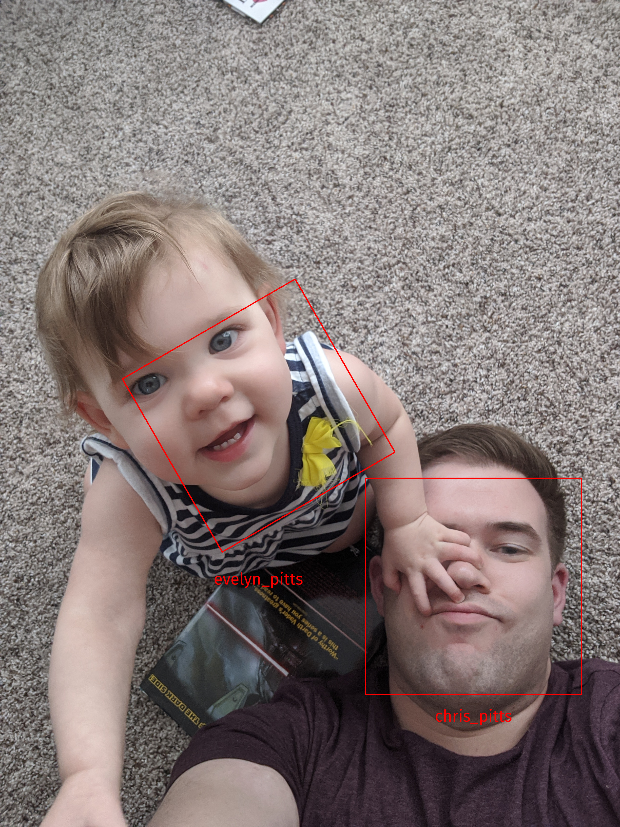
This is pretty straightforward, with one wrinkle, as noted above: sufficienty rotated faces are not identified using Haar features or classified correctly using the feature descriptors.
Finding rotated faces
One immediate problem that had to be solved was what to do about rotated faces. HOG features are not rotationally-invariant. Rotational invariance is a property of functions or algorithms where the output doesn’t change when the input is rotated. HOG features, as just noted, do not have this property, so an upside-down face won’t produce the same values as a right-side-up face. It’s tempting to think “faces will be mostly right-side up anyway,” but two problems with that line of thinking:
- Plenty of faces are “upside-down” from the perspective of the camera. Anyone who has taken pictures of a child has almost certainly gotten pictures where the face is upside down (sometimes even covered in spaghetti sauce).
- Right-side-up turns out to encompass a lot of latitude. Tilting your head by five degrees isn’t a lot, and almost everyone would say the head is right-side up, but that will still produce different feature descriptors.
To detect rotated faces, the images are rotated by a step size (I used 15 degrees), skipping any rotations that didn’t detect a face:
        all_detections = []

        for theta in np.arange(0, 360, 15):
            tform = make_rotation_transform(img.shape, theta)
            img_rot = warp(img, tform)
            detections = detector.detect_multi_scale(
                img_rot,
                scale_factor=1.1,
                step_ratio=2.0,
                min_size=(100, 100),
                max_size=(2000, 2000),
            )

            if not detections:
                continue
The rotational transform is computed using a function based on scikit-learn’s image rotation method, but much simpler (since I don’t need to rotate around arbitrary points):
def make_rotation_transform(
    shape: Tuple[int, int, int], theta: float
) -> SimilarityTransform:
    """ Create rotation transform

    Based on scikit-image's rotate method, but only computes a simple
    rotation transform around the center of the image.

    Args:
      shape (Tuple[int, int, int]): Shape of image
      theta (float): Angle of rotation

    Returns:
      tform (SimilarityTransform): Rotation transform around center of image
    """
    rows, cols = shape[0], shape[1]

    center = np.array((cols, rows)) / 2.0 - 0.5
    tform1 = SimilarityTransform(translation=center)
    tform2 = SimilarityTransform(rotation=np.deg2rad(theta))
    tform3 = SimilarityTransform(translation=-center)
    tform = tform3 + tform2 + tform1

    tform.params[2] = (0, 0, 1)

    return tform
Predicting labels with models
Now that we can find rotated faces, we have to predict what the label should be. My strategy for doing this is to ask each of the binary classifiers if they accept the image, and if more than one accepts, to try and determine which rotation is the “best” rotation. Support vector machines don’t have a readily usable confidence metric to get a sense of how certain a model is about a prediction, but one numeric attribute they do have that can be calculated for each prediction is distance from the hyperplane. This is not a true confidence metric; there’s no intuitive reason to assume that being “far” from the hyperplane implies greater certainty compared to being “close” to the hyperplane.
def predict(
    chip: np.ndarray, models: List[Tuple[BaseEstimator, Dict[str, Any]]]
) -> Tuple[str, float]:
    """ Predict label for chip

    Iterates over trained models and appends any positive labels
    to the list, then returns the most certain prediction, as
    determined by the decision function, which computes the distance
    from the hyperplane optimized by the SVM model.

    If no model predicts a positive label, then an 'unknown' label
    is returned, along with an np.nan distance, to make sure this
    prediction is never the best in a group.

    Args:
      chip (np.ndarray): Image chip with face detection
      models (List[Tuple[BaseEstimator, Dict[str, Any]]]):
        Trained SVM models with metadata for feature extraction

    Returns:
      Tuple[str, float]: Predicted label and distance from hyperplane
    """
    chip_original = chip.copy()

    predictions = []

    for model, meta in models:
        model_chip = chip_original.copy()
        resized_chip = resize(
            model_chip, (meta["images"]["height"], meta["images"]["width"])
        )
        features = hog(
            resized_chip,
            orientations=meta["hog"]["orientations"],
            pixels_per_cell=meta["hog"]["ppc"],
            cells_per_block=meta["hog"]["cpb"],
        ).reshape(1, -1)

        if model.predict(features):
            predictions.append((meta["name"], model.decision_function(features)[0]))

    if predictions:
        return max(predictions, key=lambda x: x[1])

    return "unknown", np.nan
Labeling images
The image labeling process is fairly simple: given the label and the location, put a box around it. However, there is a complication: we can find rotated faces, but the same face could be found multiple times.
Dealing with multiple detections
The same face could be found at 0, 15, and 345 degree angles, so which one should be chosen and boxed? For this we need some metric to select a “best” box. As noted above, this isn’t really a confidence metric. But, for the purposes of having a deterministic way of deciding which box to use, it’s not obviously wrong to say “these are all the same picture, rotated in different ways, so the one that produces a larger response value is going to be the better version”.
Once face rotation and multiple detections are handled, this is how the picture of me and Evelyn gets labeled: